Multiscale heat transfer
This example shows a multiscale approach to stationary heat transfer in a perforated ceramic sheet. The sheet has a periodic structure, so it is advantageous to separate two scales:
- Macroscale: the ceramic sheet measures 400 × 200 mm and contains circular holes. The heat transfer model replaces this heterogeneous morphology with a homogeneous continuum, using an effective conductivity obtained from the microscale.
- Microscale: a representative volume element (RVE) of 2 × 2 mm captures the morphology of the sheet around one circular hole. The effective conductivity of the RVE is computed.
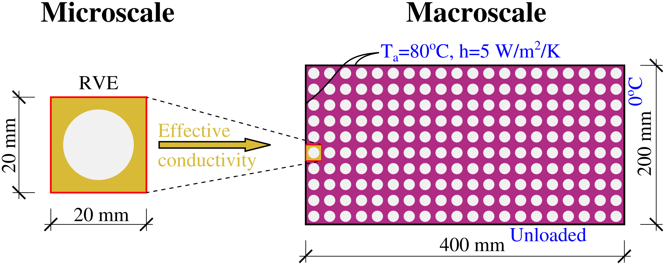
Microscale
The RVE is loaded by a temperature gradient in the x direction: 0 °C on the left edge and 1 °C on the right edge. It uses a regular mesh of 40 × 40 quadrilateral elements, which gives 1599 equations, with a heat conductivity of 1.0 W/m/K for the solid. The effective conductivity is obtained from the heat flow through the right edge and the prescribed boundary temperatures. It evaluates to 0.314 W/m/K.
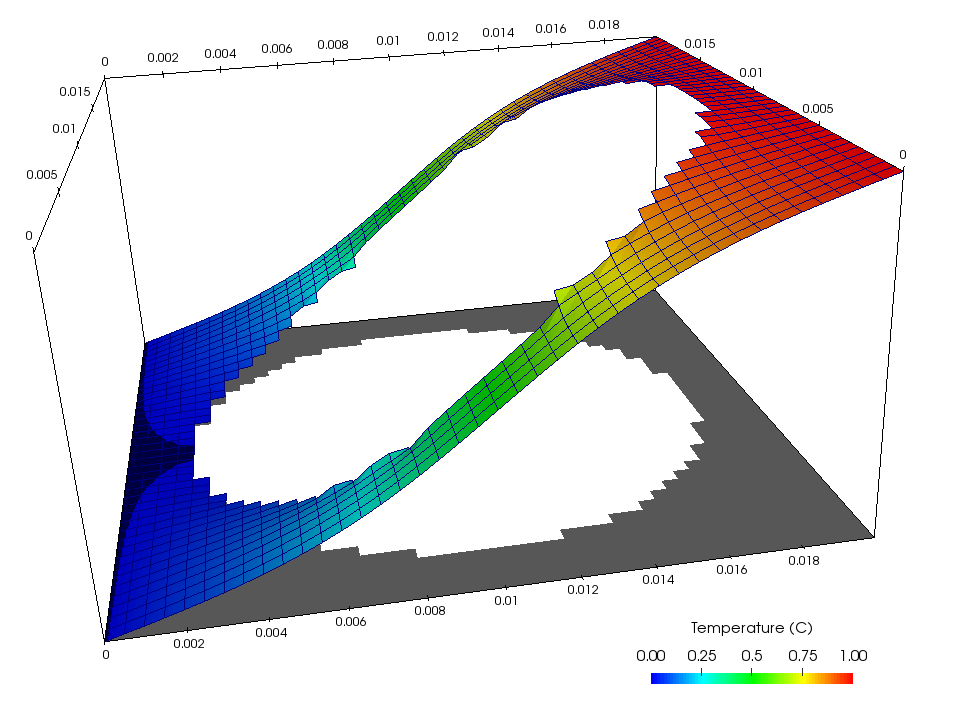
Macroscale
The effective conductivity is passed to the macroscale model, which is discretized into 40 × 20 finite elements (840 equations).
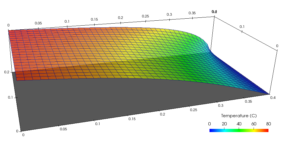
The workflow
import mupif as mp

# microscale: compute the effective conductivity of the RVE
micro.solveStep(tstep)
k_eff = micro.get(mp.DataID.PID_effective_conductivity, tstep.getTime())

# macroscale: use it as the material property of the homogenized sheet
macro.set(k_eff)
macro.solveStep(tstep)
temperature = macro.get(mp.DataID.FID_Temperature, tstep.getTime())
The two models only exchange a Property object with its units, so either model can be
replaced, for example by a different solver or by an RVE model running on HPC, without
changing the other.
 (since February, 2023)